Tutorial 3: Xenium Prime 5K: Mouse Brain
Analyze mouse brain spatial transcriptomics data with SpacGPA.
Data source: https://www.10xgenomics.com/datasets/xenium-prime-fresh-frozen-mouse-brain
This is a mouse brain sample generated with Xenium Prime 5K.
[1]:
# Import SpacGPA and other required packages.
import SpacGPA as sg
import scanpy as sc
import matplotlib.pyplot as plt
import pandas as pd
import os
[2]:
# Set the working directory to your local path.
workdir = '..'
os.chdir(workdir)
Part 1: Gene program analysis via SpacGPA
[3]:
# Load spatial transcriptomics data.
# Read the count matrix from the 10x Genomics Cell Ranger output.
adata = sc.read_10x_h5('data/Xenium_5k/Mouse_Brain_5K/cell_feature_matrix.h5')
adata.var_names_make_unique()
adata.var_names = adata.var['gene_ids']
# Read the cell metadata (including spatial coordinates) from the provided CSV file.
meta = pd.read_csv('data/Xenium_5k/Mouse_Brain_5K/cells.csv.gz')
meta.index = meta['cell_id'].astype(str)
meta = meta.reindex(adata.obs_names)
adata.obs = adata.obs.join(meta, how='left')
# Set the spatial coordinates.
adata.obsm['spatial'] = adata.obs[['y_centroid','x_centroid']].values*[-1,-1]
print(adata)
AnnData object with n_obs × n_vars = 63173 × 5006
    obs: 'cell_id', 'x_centroid', 'y_centroid', 'transcript_counts', 'control_probe_counts', 'genomic_control_counts', 'control_codeword_counts', 'unassigned_codeword_counts', 'deprecated_codeword_counts', 'total_counts', 'cell_area', 'nucleus_area', 'nucleus_count', 'segmentation_method'
    var: 'gene_ids', 'feature_types', 'genome'
    obsm: 'spatial'
[4]:
# Preprocessing: log1p-transform.
sc.pp.log1p(adata)
sc.pp.filter_cells(adata, min_genes=100)
sc.pp.filter_genes(adata, min_cells = 10)
print(adata.X.shape)
(62207, 5002)
[5]:
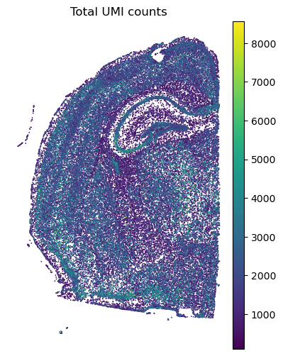
# Visualize the total UMI counts per spot.
plt.rcParams["figure.figsize"] = (4.5, 6)
sc.pl.spatial(adata, spot_size = 30, color = 'total_counts', frameon = False, title = 'Total UMI counts')
[6]:
# Construct the co-expression network using SpacGPA (Gaussian graphical model).
ggm = sg.create_ggm(adata, project_name = "Mouse Brain")
Please Normalize The Expression Matrix Before Running!
Loading Data.

Running all calculations on GPU (if available).
Using single precision (float32) for all calculations.
Using chunk size of 5000 for efficient computation

Computing the number of cells co-expressing each gene pair...
Computing covariance matrix...
Computing Pearson correlation matrix...

Calculating partial correlations in 2498 iterations.
Number of genes randomly selected in each iteration: 1001
Iteration: 2498/2498, Avg loop time: 0.0126 s, Elapsed time: 0.56 min, Estimated time left: 0.00 min.
All iterations completed.

Performing FDR control...
Randomly redistribute the expression distribution of input genes...

Calculate correlation between genes after redistribution...

Computing the number of cells co-expressing each gene pair...
Computing covariance matrix...
Computing Pearson correlation matrix...

Calculating partial correlations in 2498 iterations.
Number of genes randomly selected in each iteration: 1001
Iteration: 2498/2498, Avg loop time: 0.0126 s, Elapsed time: 0.53 min, Estimated time left: 0.00 min.
All iterations completed.

Summarizing the FDR Statistics...
FDR control completed.
Current Pcor threshold: 0.020
Minimum Pcor threshold with FDR <= 0.05: 0.013
FDR at pcor=0.02: 8.71e-04

Task completed. Resources released.
[7]:
# Show statistically significant co-expression gene pairs.
print(ggm.SigEdges.head(5))
                GeneA               GeneB      Pcor  SamplingTime         r  \
0  ENSMUSG00000029802  ENSMUSG00000040584  0.096567            90  0.578254
1  ENSMUSG00000029802  ENSMUSG00000030834  0.031893            89  0.231888
2  ENSMUSG00000020681  ENSMUSG00000028125  0.042191           118  0.442514
3  ENSMUSG00000015405  ENSMUSG00000030249  0.095438           100  0.511198
4  ENSMUSG00000044337  ENSMUSG00000015405  0.029435           108  0.242722

   Cell_num_A  Cell_num_B  Cell_num_coexpressed      Project
0        7142        7338                  3822  Mouse Brain
1        7142         925                   573  Mouse Brain
2        2258        1164                   360  Mouse Brain
3        1131        1067                   507  Mouse Brain
4        4151        1131                   462  Mouse Brain
[8]:
# Identify gene programs using the MCL-Hub algorithm (set inflation to 2).
ggm.find_modules(method = 'mcl-hub', inflation = 2, convert_to_symbols = True, species = 'mouse')
# the parameter 'convert_to_symbols' provides gene symbols in the output programs for better interpretability.
Find modules using MCL-Hub...
Current Pcor: 0.02
Total significantly co-expressed gene pairs: 39055
Iteration: 29, Max change: 0.00000000
Converged at iteration 29.

0 modules were removed due to their linear or radial topology structure out of 70 modules.

Converting Ensembl IDs to gene symbols...
[9]:
# Inspect the top 5 identified gene programs.
print(ggm.modules_summary.head(5))
  module_id  size  num_genes_degree_ge_2  \
0        M1   140                    130
1        M2   131                    120
2        M3   118                    103
3        M4   109                     98
4        M5   100                     94

                                         all_symbols  \
0  P2ry13, Il10ra, Cx3cr1, Selplg, Vsir, Csf3r, T...
1  Slc7a10, Lfng, Agt, Gjb6, S1pr1, Slc6a11, Fgfr...
2  Slc47a1, Thbs1, Foxc2, Cdh1, Eya2, Col6a2, Bnc...
3  Spink8, Fibcd1, Neurod6, Scn3b, Iqgap2, Gria1,...
4  Flt1, Abcb1a, Pltp, Esam, Adgrf5, Sox18, Eng, ...

                                           all_genes
0  ENSMUSG00000036362, ENSMUSG00000032089, ENSMUS...
1  ENSMUSG00000030495, ENSMUSG00000029570, ENSMUS...
2  ENSMUSG00000010122, ENSMUSG00000040152, ENSMUS...
3  ENSMUSG00000050074, ENSMUSG00000026841, ENSMUS...
4  ENSMUSG00000029648, ENSMUSG00000040584, ENSMUS...
[10]:
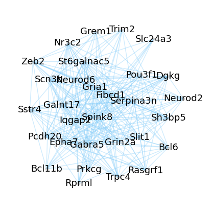
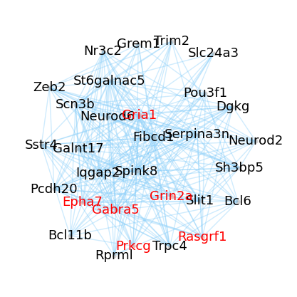
# Visualize the subnetwork of program M4 (top 30 genes by degree/connectivity for readability).
ggm.module_network_plot(module_id = 'M4', seed = 2, layout_iterations = 60)
# Fix layout randomness for reproducibility via set seed.
[11]:
# Gene Ontology (GO) enrichment analysis with BH FDR control and p-value threshold 0.05.
ggm.go_enrichment_analysis(species = 'mouse', padjust_method = "BH", pvalue_cutoff = 0.05)
Reading GO term information for |mouse|...

Start GO enrichment analysis ...
Found 0 significant enriched GO terms in M70
GO enrichment analysis completed. Found 4538 significant enriched GO terms total.
[ ]:
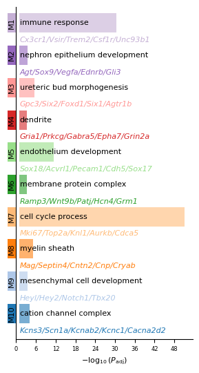
# Visualize top enriched GO terms for top 10 identified programs.
program_list = ggm.modules_summary['module_id'].tolist()
ggm.module_go_enrichment_plot(shown_modules = program_list[:10], go_per_module = 1)
[13]:
# Mammalian Phenotype (MP) Ontology enrichment analysis with BH FDR control and p-value threshold 0.05.
ggm.mp_enrichment_analysis(species = 'mouse', padjust_method = "BH", pvalue_cutoff = 0.05)
Reading MP term information for |mouse|...

Start MP enrichment analysis ...
Found 0 significant enriched MP terms in M70
MP enrichment analysis completed. Found 2609 significant enriched MP terms total.
[ ]:
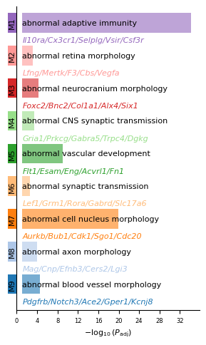
# Visualize top enriched MP terms for top 10 identified programs.
ggm.module_mp_enrichment_plot(shown_modules = program_list[:10], mp_per_module = 1)
[15]:
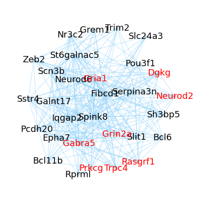
# Visualize the M4 network with nodes highlighted by a selected GO or MP term.
M4_GO_Enrich = ggm.go_enrichment[ggm.go_enrichment['module_id'] == 'M4']
print(M4_GO_Enrich.iloc[:3, :6])
ggm.module_network_plot(module_id = 'M4', highlight_anno = "dendrite", seed = 2, layout_iterations = 55)
M4_MP_Enrich = ggm.mp_enrichment[ggm.mp_enrichment['module_id'] == 'M4']
print(M4_MP_Enrich.iloc[:3, :5])
ggm.module_network_plot(module_id = 'M4', highlight_anno = "abnormal CNS synaptic transmission", seed = 2, layout_iterations = 55)
    module_id  module_size  go_rank       go_id         go_category  \
970        M4          109        1  GO:0030425  cellular_component
971        M4          109        2  GO:0097447  cellular_component
972        M4          109        3  GO:0098794  cellular_component

            go_term
970        dendrite
971  dendritic tree
972     postsynapse
    module_id  module_size  mp_rank       mp_id  \
730        M4          109        1  MP:0002206
731        M4          109        2  MP:0003635
732        M4          109        3  MP:0021009

                                mp_term
730  abnormal CNS synaptic transmission
731      abnormal synaptic transmission
732        abnormal synaptic physiology
[16]:
# Print a summary of the GGM analysis.
print(ggm)
View of ggm object: Mouse Brain
MetaInfo:
  Gene Number: 5002
  Sample Number: 62207
  Pcor Threshold: 0.02

Results:
  SigEdges: DataFrame with 39055 significant gene pairs
  modules: 70 modules with 2825 genes
  modules_summary: DataFrame with 70 rows
  FDR: Exists
[17]:
# Save the GGM object to HDF5 for later reuse.
sg.save_ggm(ggm, "data/Mouse_Brain_5K.ggm.h5")
Part 2: Spot annotation based on program expression
[18]:
# Compute per-spot expression scores of each gene program.
sg.calculate_module_expression(adata, ggm)
Calculating module expression using top 30 genes...

Calculating gene weights based on degree...
Storing module information in adata.uns['module_info']...

Assigning colors to 70 modules...

Total 70 modules' average expression calculated and stored in adata.obs and adata.obsm
[19]:
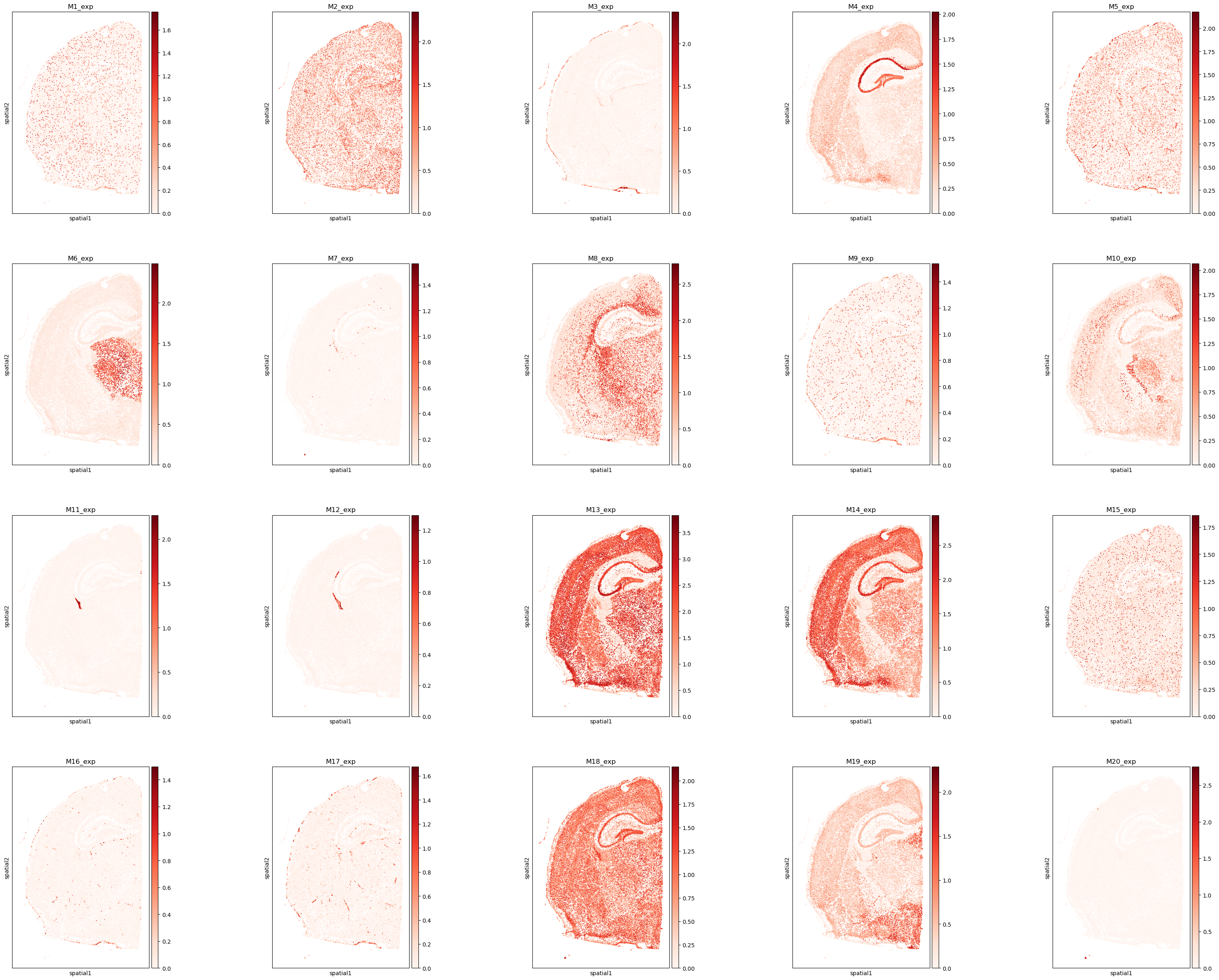
# Visualize the spatial distribution of the top 20 program-expression scores.
plt.rcParams["figure.figsize"] = (7, 7)
program_list = ggm.modules_summary['module_id'] + '_exp'
sc.pl.spatial(adata, spot_size = 30, color = program_list[:20], cmap = 'Reds', ncols = 5)
[20]:
# Compute pairwise program similarity and plot the correlation heatmap with dendrograms.
sg.module_similarity_plot(adata, ggm_key = 'ggm', corr_method = 'pearson', heatmap_metric = 'correlation',
                          fig_height = 19, fig_width = 20, dendrogram_height = 0.1, dendrogram_space = 0.06, return_summary = False)

[21]:
# Assign spot-level annotations via Gaussian Mixture Models (GMMs) based on program expression.
sg.calculate_gmm_annotations(adata, ggm_key = 'ggm')
M1 processed successfully, annotated cells: 4359
M2 processed successfully, annotated cells: 9347
M3 processed successfully, annotated cells: 2512
M4 processed successfully, annotated cells: 20517
M5 processed successfully, annotated cells: 9304
M6 processed successfully, annotated cells: 3587
M7 processed successfully, annotated cells: 346
M8 processed successfully, annotated cells: 8198
M9 processed successfully, annotated cells: 4330
M10 processed successfully, annotated cells: 2501
M11 processed successfully, annotated cells: 794
M12 processed successfully, annotated cells: 465
M13 processed successfully, annotated cells: 26976
M14 processed successfully, annotated cells: 23015
M15 processed successfully, annotated cells: 2192
M16 processed successfully, annotated cells: 2498
M17 processed successfully, annotated cells: 4120
M18 processed successfully, annotated cells: 1336
M19 processed successfully, annotated cells: 18649
M20 processed successfully, annotated cells: 53
M21 processed successfully, annotated cells: 1406
M22 processed successfully, annotated cells: 725
M23 processed successfully, annotated cells: 2639
M24 processed successfully, annotated cells: 2684
M25 processed successfully, annotated cells: 2383
M26 processed successfully, annotated cells: 4845
M27 processed successfully, annotated cells: 1953
M28 processed successfully, annotated cells: 2609
M29 processed successfully, annotated cells: 410
M30 processed successfully, annotated cells: 2929
M31 processed successfully, annotated cells: 1703
M32 processed successfully, annotated cells: 5086
M33 processed successfully, annotated cells: 14982
M34 processed successfully, annotated cells: 10133
M35 processed successfully, annotated cells: 29311
M36 processed successfully, annotated cells: 8941
M37 processed successfully, annotated cells: 11138
M38 processed successfully, annotated cells: 1969
M39 processed successfully, annotated cells: 1505
M40 processed successfully, annotated cells: 3988
M41 processed successfully, annotated cells: 1950
M42 processed successfully, annotated cells: 1861
M43 processed successfully, annotated cells: 3918
M44 processed successfully, annotated cells: 2151
M45 processed successfully, annotated cells: 48
M46 processed successfully, annotated cells: 3333
M47 processed successfully, annotated cells: 52
M48 processed successfully, annotated cells: 1909
M49 processed successfully, annotated cells: 1823
M50 processed successfully, annotated cells: 2008
M51 processed successfully, annotated cells: 21935
M52 processed successfully, annotated cells: 14768
M53 processed successfully, annotated cells: 13827
M54 processed successfully, annotated cells: 4273
M55 processed successfully, annotated cells: 54
M56 processed successfully, annotated cells: 2241
M57 processed successfully, annotated cells: 2608
M58 processed successfully, annotated cells: 2819
M59 processed successfully, annotated cells: 505
M60 processed successfully, annotated cells: 63
M61 processed successfully, annotated cells: 483
M62 processed successfully, annotated cells: 1296
M63 processed successfully, annotated cells: 1695
M64 processed successfully, annotated cells: 9711
M65 processed successfully, annotated cells: 1596
M66 processed successfully, annotated cells: 2445
M67 processed successfully, annotated cells: 1469
M68 processed successfully, annotated cells: 9558
M69 processed successfully, annotated cells: 2280
M70 processed successfully, annotated cells: 5247
[22]:
# Optionally smooth the annotations using spatial k-NN (on the 'spatial' embedding).
sg.smooth_annotations(adata, ggm_key = 'ggm', embedding_key = 'spatial', k_neighbors = 24)
M1 processed. remain cells: 3752
M2 processed. remain cells: 9435
M3 processed. remain cells: 2893
M4 processed. remain cells: 26876
M5 processed. remain cells: 9905
M6 processed. remain cells: 5146
M7 processed. remain cells: 270
M8 processed. remain cells: 9144
M9 processed. remain cells: 4475
M10 processed. remain cells: 2142
M11 processed. remain cells: 815
M12 processed. remain cells: 612
M13 processed. remain cells: 39646
M14 processed. remain cells: 32708
M15 processed. remain cells: 1369
M16 processed. remain cells: 1796
M17 processed. remain cells: 3765
M18 processed. remain cells: 775
M19 processed. remain cells: 23926
M20 processed. remain cells: 45
M21 processed. remain cells: 896
M22 processed. remain cells: 694
M23 processed. remain cells: 3810
M24 processed. remain cells: 3126
M25 processed. remain cells: 2492
M26 processed. remain cells: 4528
M27 processed. remain cells: 1140
M28 processed. remain cells: 2430
M29 processed. remain cells: 171
M30 processed. remain cells: 2847
M31 processed. remain cells: 1295
M32 processed. remain cells: 5787
M33 processed. remain cells: 18553
M34 processed. remain cells: 12815
M35 processed. remain cells: 39652
M36 processed. remain cells: 9448
M37 processed. remain cells: 13302
M38 processed. remain cells: 1618
M39 processed. remain cells: 960
M40 processed. remain cells: 3422
M41 processed. remain cells: 1903
M42 processed. remain cells: 1302
M43 processed. remain cells: 4542
M44 processed. remain cells: 2414
M45 processed. remain cells: 47
M46 processed. remain cells: 3418
M47 processed. remain cells: 11
M48 processed. remain cells: 1329
M49 processed. remain cells: 2240
M50 processed. remain cells: 1495
M51 processed. remain cells: 30415
M52 processed. remain cells: 16658
M53 processed. remain cells: 15532
M54 processed. remain cells: 5045
M55 processed. remain cells: 13
M56 processed. remain cells: 2720
M57 processed. remain cells: 2636
M58 processed. remain cells: 3025
M59 processed. remain cells: 327
M60 processed. remain cells: 11
M61 processed. remain cells: 340
M62 processed. remain cells: 1001
M63 processed. remain cells: 1168
M64 processed. remain cells: 11111
M65 processed. remain cells: 1283
M66 processed. remain cells: 2025
M67 processed. remain cells: 1045
M68 processed. remain cells: 11221
M69 processed. remain cells: 2120
M70 processed. remain cells: 5259

Annotation smoothing completed. Results stored in adata.obs.
[23]:
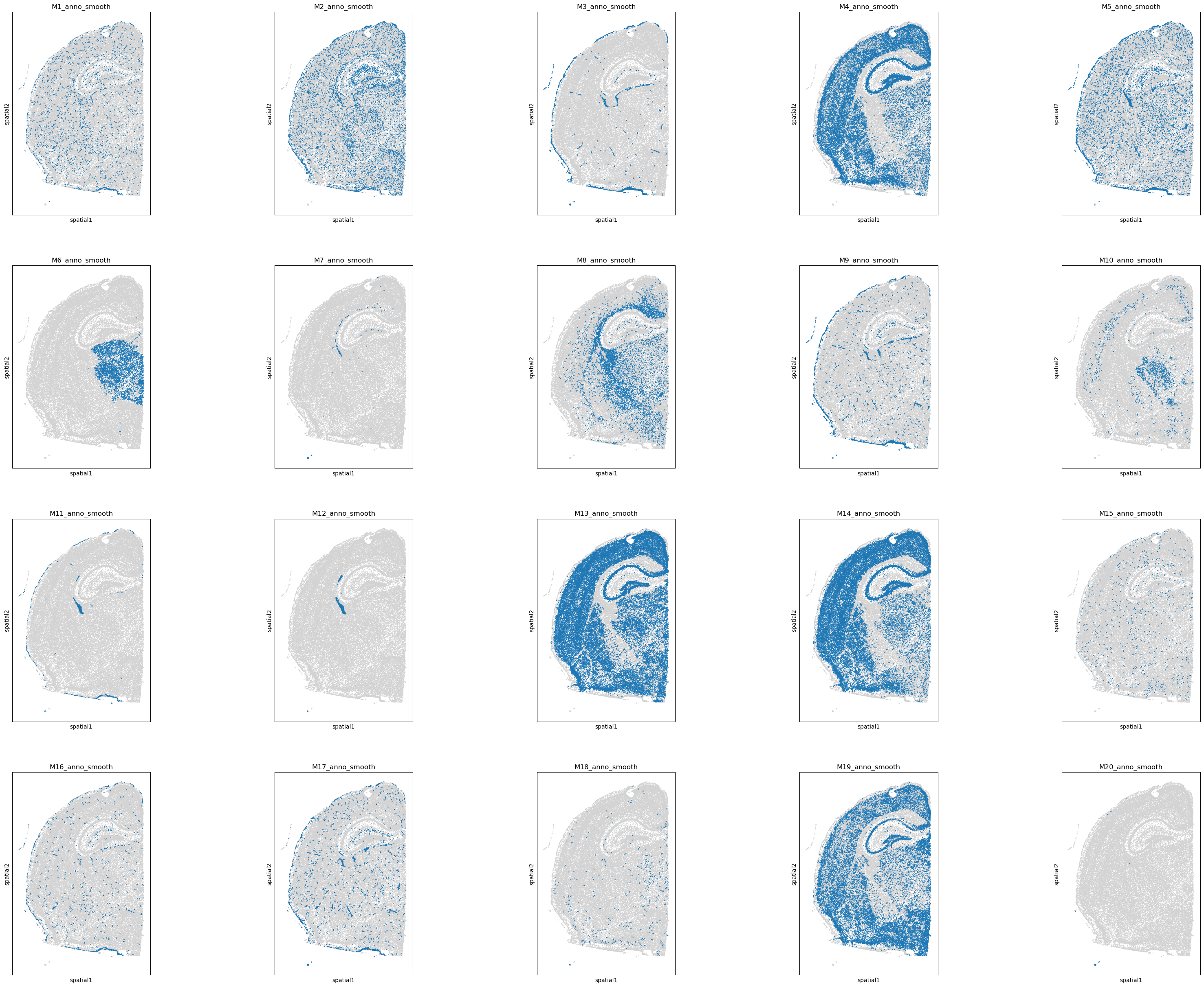
# Display smoothed annotations for top 20 programs.
# If smoothing is skipped, use 'M1_anno' … 'M20_anno' instead.
program_list = ggm.modules_summary['module_id'] + '_anno_smooth'
sc.pl.spatial(adata, spot_size = 30, color = program_list[:20], legend_loc = None, ncols = 5)
# Where the blue nodes indicate the spots annotated by the program, and gray nodes are unassigned.
[24]:
# Integrate multiple program-derived annotations into a single label set via sg.integrate_annotations.
sg.integrate_annotations(adata, ggm_key = 'ggm', use_smooth = False, neighbor_similarity_ratio = 0.6, result_anno = 'ggm_annotation')
# Here we integrate all programs as an example. You can specify a subset of programs via the 'modules_used' parameter.
Calculating 24 nearest neighbors for each cell based on spatial embedding...


51059 of total 62207 cells have multiple annotations. Among them,
    7317 cells are resolved by neighbors.
    43742 cells are resolved by expression score.

Integrated annotation stored in adata.obs['ggm_annotation'].
[25]:
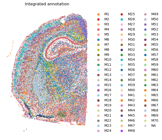
# Visualize the integrated annotation.
plt.rcParams["figure.figsize"] = (7, 7)
sc.pl.spatial(adata, spot_size = 30, color = ['ggm_annotation'], palette = adata.uns['module_colors'], frameon = False, title = 'Integrated annotation')
Part 3: Cluster spots based a dimensionality reduction of program expression
[26]:
# Build a neighborhood graph based on program expression and perform clustering.
sc.pp.neighbors(adata,
                use_rep='module_expression_scaled',
                n_pcs=adata.obsm['module_expression_scaled'].shape[1])
sc.tl.leiden(adata, resolution=3, key_added='leiden_ggm')
sc.tl.louvain(adata, resolution=3, key_added='louvan_ggm')
[27]:
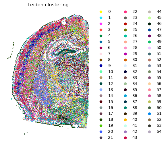
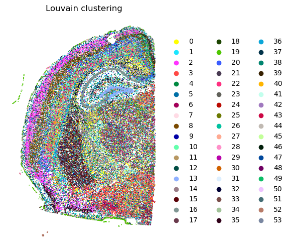
# Visualize the clustering results.
plt.rcParams["figure.figsize"] = (6, 6)
sc.pl.spatial(adata, spot_size = 30, color = ['leiden_ggm'], frameon = False, title = 'Leiden clustering')
plt.rcParams["figure.figsize"] = (6, 6)
sc.pl.spatial(adata, spot_size = 30, color = ['louvan_ggm'], frameon = False, title = 'Louvain clustering')
[28]:
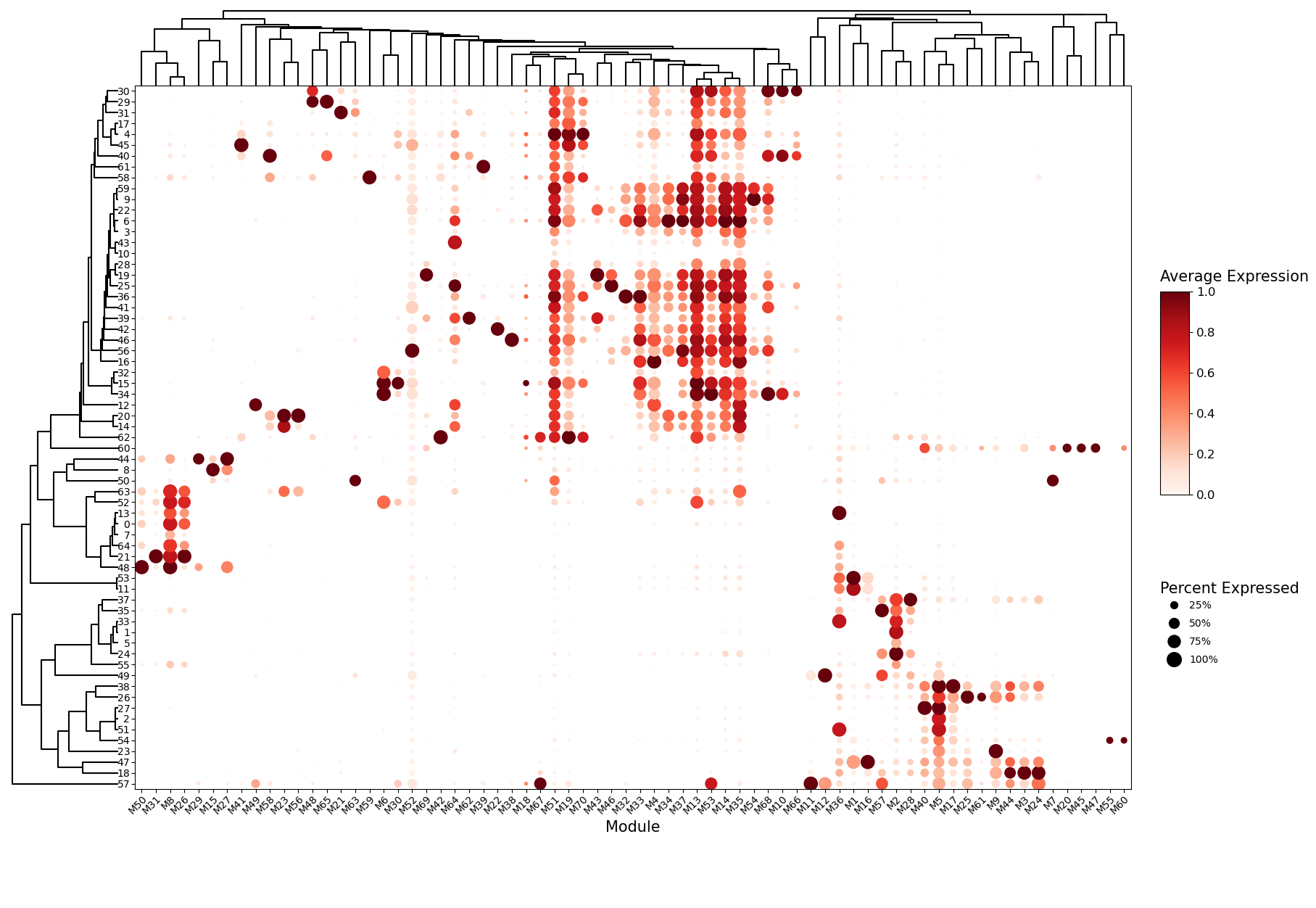
# Summarize program-expression across the leiden clusters clusters as a dot plot.
sg.module_dot_plot(adata, ggm_key = 'ggm', groupby = 'leiden_ggm', scale=True,
                   dendrogram_height = 0.1, dendrogram_space = 0.03, fig_height=14, fig_width = 20, axis_fontsize = 10)
[29]:
# Save the annotated AnnData object.
adata.write("data/Mouse_Brain_5K_ggm_anno.h5ad")