Tutorial 6: Atera: Breast Tumor
Analyze 10x Atera breast tumor spatial transcriptomics data with SpacGPA.
The Atera data folder used in this tutorial contains three required files: cell_feature_matrix.h5, cells.csv.gz, and cell_boundaries.csv.gz.
[1]:
# Import SpacGPA and other required packages.
import SpacGPA as sg
import scanpy as sc
import matplotlib.pyplot as plt
import os
import warnings
warnings.filterwarnings('ignore', message=r'.*Variable names are not unique.*')
[2]:
# Set the working directory to your local path.
workdir = '..'
os.chdir(workdir)
Part 1: Gene program analysis via SpacGPA
[3]:
# Load Atera data.
adata = sg.load_atera('data/Atera/Breast_Tumor')
print(adata)
AnnData object with n_obs × n_vars = 170057 × 18028
    obs: 'x_centroid', 'y_centroid', 'transcript_counts', 'control_probe_counts', 'genomic_control_counts', 'control_codeword_counts', 'unassigned_codeword_counts', 'deprecated_codeword_counts', 'total_counts', 'cell_area', 'nucleus_area', 'nucleus_count', 'segmentation_method', 'polygon'
    var: 'gene_ids', 'feature_types', 'genome'
    obsm: 'spatial'
[4]:
# Preprocessing: library-size normalize and log1p-transform.
sc.pp.filter_cells(adata, min_counts=1)
sc.pp.normalize_total(adata, target_sum = 1e4)
sc.pp.log1p(adata)
sc.pp.filter_cells(adata, min_genes = 200)
sc.pp.filter_genes(adata, min_cells = 10)
print(adata.X.shape)
(165301, 18022)
[5]:
# Construct the co-expression network using SpacGPA (Gaussian graphical model).
ggm = sg.create_ggm(adata, project_name = 'Breast Tumor')
Please Normalize The Expression Matrix Before Running!
Loading Data.

Running all calculations on GPU (if available).
Using single precision (float32) for all calculations.
Using chunk size of 5000 for efficient computation

Computing the number of cells co-expressing each gene pair...
Computing covariance matrix...
Computing Pearson correlation matrix...

Calculating partial correlations in 8120 iterations.
Number of genes randomly selected in each iteration: 2000
Iteration: 8120/8120, Avg loop time: 0.0372 s, Elapsed time: 5.15 min, Estimated time left: 0.00 min.
All iterations completed.

Performing FDR control...
Randomly redistribute the expression distribution of input genes...

Calculate correlation between genes after redistribution...

Computing the number of cells co-expressing each gene pair...
Computing covariance matrix...
Computing Pearson correlation matrix...

Calculating partial correlations in 8120 iterations.
Number of genes randomly selected in each iteration: 2000
Iteration: 8120/8120, Avg loop time: 0.0371 s, Elapsed time: 5.12 min, Estimated time left: 0.00 min.
All iterations completed.

Summarizing the FDR Statistics...
FDR control completed.
Current Pcor threshold: 0.020
Minimum Pcor threshold with FDR <= 0.05: 0.010
FDR at pcor=0.02: 0.00e+00

Task completed. Resources released.
[6]:
# Show statistically significant co-expression gene pairs.
print(ggm.SigEdges.head(5))
    GeneA   GeneB      Pcor  SamplingTime         r  Cell_num_A  Cell_num_B  \
0  ABCA10    AASS  0.021785           110  0.140313       17773       22553
1   ABCA6    AASS  0.026992            94  0.161891       30479       22553
2   ABCA6  ABCA10  0.170752           104  0.504233       30479       17773
3   ABCA8  ABCA10  0.096947           132  0.373468       21301       17773
4   ABCA8   ABCA6  0.097767           109  0.433015       21301       30479

   Cell_num_coexpressed       Project
0                  4225  Breast Tumor
1                  6462  Breast Tumor
2                 10677  Breast Tumor
3                  7385  Breast Tumor
4                 11000  Breast Tumor
[7]:
# Identify gene programs using the MCL-Hub algorithm (set inflation to 2).
ggm.find_modules(method = 'mcl-hub', inflation = 2)
Find modules using MCL-Hub...
Current Pcor: 0.02
Total significantly co-expressed gene pairs: 64309
Iteration: 29, Max change: 0.00000000
Converged at iteration 29.

2 modules were removed due to their linear or radial topology structure out of 108 modules.
[8]:
# Inspect the top 5 identified gene programs.
print(ggm.modules_summary.head(5))
  module_id  size  num_genes_degree_ge_2  \
0        M1   306                    239
1        M2   287                    251
2        M3   241                    207
3        M4   220                     32
4        M5   196                    161

                                           all_genes
0  GABRP, PROM1, CCL28, KRT15, KRT23, KIT, KLK5, ...
1  TRAC, CD3E, ACAP1, TMC8, CD52, TRBC2, ZAP70, S...
2  TNS4, COL17A1, MYLK, TP63, TAGLN, LAMB3, LTBP2...
3  SMG1, PKD1, EME2, SULT1A1, SNX29, MAPK8IP3, C1...
4  BTNL9, KDR, SHANK3, EXOC3L2, FLT1, RGCC, APOLD...
[9]:
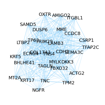
# Visualize the subnetwork of program M3.
ggm.module_network_plot(module_id = 'M3', seed = 2, layout_iterations = 60)
# Fix layout randomness for reproducibility via set seed.
[10]:
# Gene Ontology (GO) enrichment analysis with BH FDR control and p-value threshold 0.05.
ggm.go_enrichment_analysis(species = 'human', padjust_method = 'BH', pvalue_cutoff = 0.05)
Reading GO term information for |human|...

Start GO enrichment analysis ...
Found 66 significant enriched GO terms in M106
GO enrichment analysis completed. Found 7609 significant enriched GO terms total.
[11]:
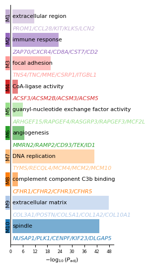
# Visualize top enriched GO terms for top 10 identified programs.
program_list = ggm.modules_summary['module_id'].tolist()
ggm.module_go_enrichment_plot(shown_modules = program_list[:10], go_per_module = 1)
[12]:
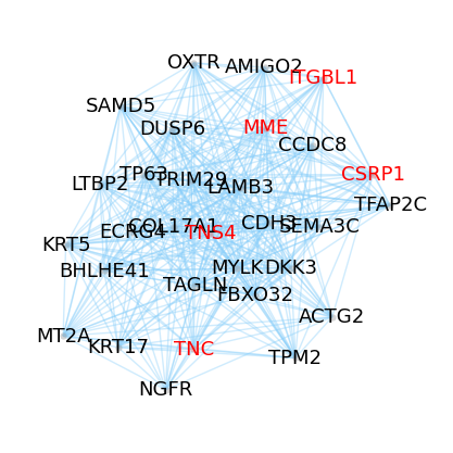
# Visualize the M3 network with nodes highlighted by a selected GO term.
M3_GO_Enrich = ggm.go_enrichment[ggm.go_enrichment['module_id'] == 'M3']
print(M3_GO_Enrich.iloc[:3, :6])
ggm.module_network_plot(module_id = 'M3', highlight_anno = 'focal adhesion', seed = 2, layout_iterations = 60)
    module_id  module_size  go_rank       go_id         go_category  \
265        M3          241        1  GO:0005925  cellular_component
266        M3          241        2  GO:0001725  cellular_component
267        M3          241        3  GO:0030018  cellular_component

            go_term
265  focal adhesion
266    stress fiber
267          Z disc
[13]:
# Print a summary of the GGM analysis.
print(ggm)
View of ggm object: Breast Tumor
MetaInfo:
  Gene Number: 18022
  Sample Number: 165301
  Pcor Threshold: 0.02

Results:
  SigEdges: DataFrame with 64309 significant gene pairs
  modules: 106 modules with 6008 genes
  modules_summary: DataFrame with 106 rows
  FDR: Exists
[14]:
# Save the GGM object to HDF5 for later reuse.
sg.save_ggm(ggm, 'data/Atera_Breast_Tumor.ggm.h5')
Part 2: Cell annotation based on program expression
[15]:
# Compute per-cell expression scores of each gene program.
sg.calculate_module_expression(adata, ggm)
Calculating module expression using top 30 genes...

Calculating gene weights based on degree...
Storing module information in adata.uns['module_info']...

Assigning colors to 106 modules...

Total 106 modules' average expression calculated and stored in adata.obs and adata.obsm
[16]:
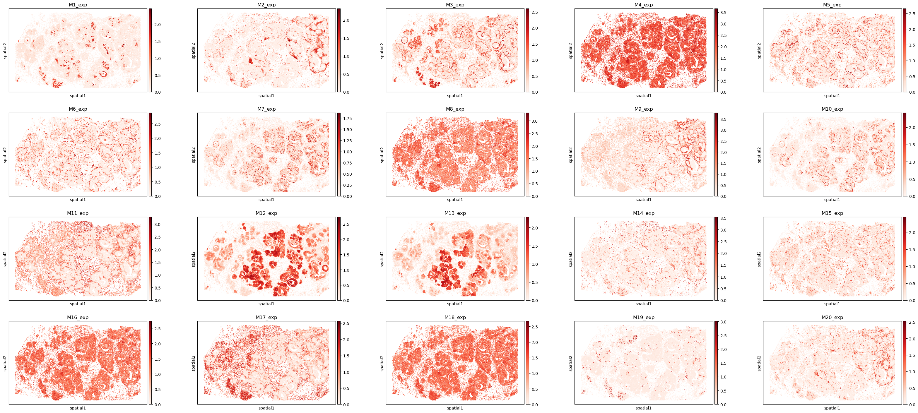
# Visualize the spatial distribution of the top 20 program-expression scores.
plt.rcParams['figure.figsize'] = (7, 4)
program_list = ggm.modules_summary['module_id'] + '_exp'
sc.pl.spatial(adata, spot_size = 30, color = program_list[:20], cmap = 'Reds', ncols = 5)
[17]:
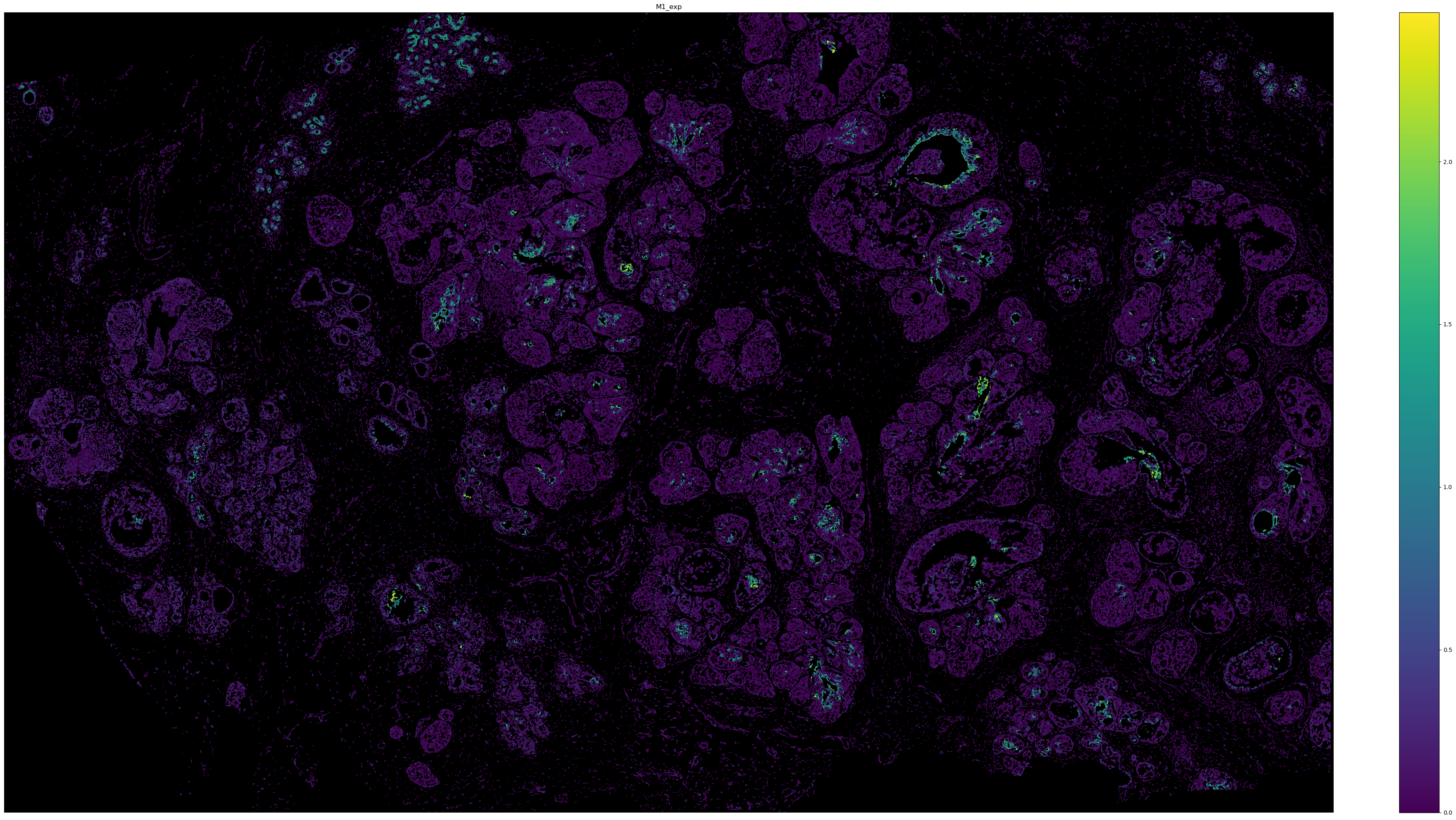
# Visualize the expression of M1 with cell boundary polygons.
sg.pl.spatial_polygon(adata, color = 'M1_exp', figsize = (40, 20), background = 'black')
[18]:
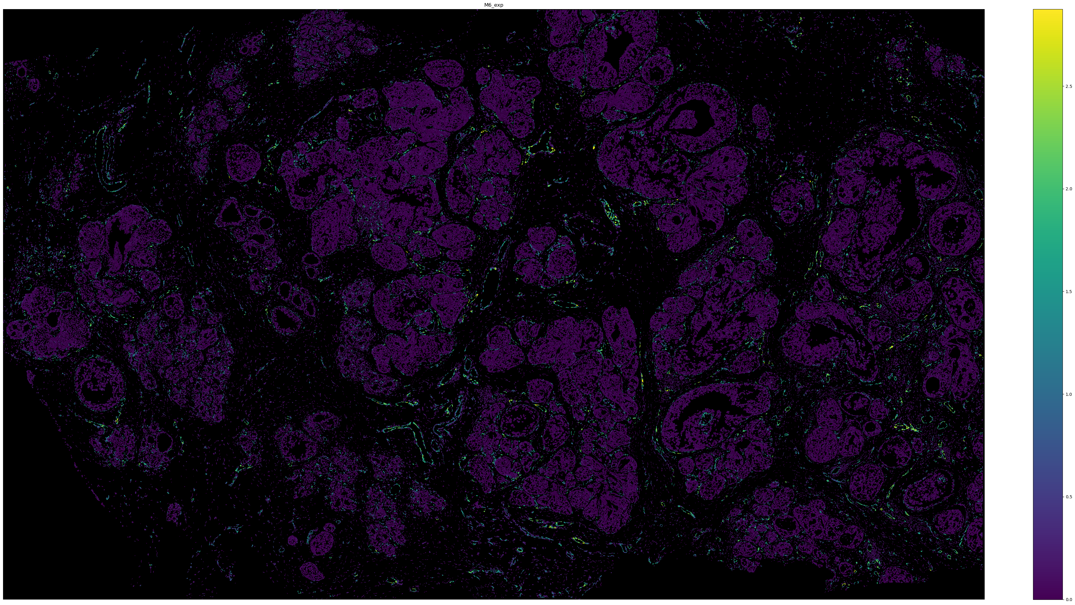
# Visualize the expression of M6 with cell boundary polygons.
sg.pl.spatial_polygon(adata, color = 'M6_exp', figsize = (40, 20), background = 'black')
[19]:
# Save the annotated AnnData object.
adata.write('data/Atera_Breast_Tumor_ggm_anno.h5ad')